My attempt to present an intuitive account of causal reasoning and the important notions of causal conditioning and counterfactuals without resorting to some of the formalities of do-calculus, d-separation, couterfactual notation and the like. All the programs in the post will be in R, but should be accessible to readers with no experience with the language.
Causal reasoning from scientific data has undergone a quiet revolution in the past couple of decades. The fundamentals of the newly clarified concepts and algorithmic frameworks for systematically answering causal questions are simple and ought to be more widely known than they are. There are several excellent expositions on the topic (some references at the bottom of the post), but perhaps another one won’t be unwelcome.
I will use a running example accompanied by simple programs in R to illustrate the concepts. First a little background to set up our example.
The amount of energy generated by photovoltaic solar power-plants is decreased by not an insignificant amount when dirt and other particulates collect on the panels. This, so-called soiling problem is especially acute in dusty desert regions which are otherwise ideal sites for solar plants, because the sun shines bright when there aren’t many clouds in sight. Consequently plant operators are always on the lookout for cheap and effective panel soiling mitigation strategies.
Imagine that a meticulous solar-scientist named Sol is tasked with estimating the effect on the energy production of weekly washing of the panels in a fleet of solar power plants. Assume that he has at hand data on weekly aggregates of days of rainfall (denoted \(R\)), weekly average cloud-cover (denoted \(C\)), and total weekly energy production from the solar fleet (denoted \(E\)). Sol reasons that if he could estimate the effect of having at least one day of rain on the amount of energy produced, he could use it as a proxy for weekly washing.
Before tackling the panel washing problem, Sol analyzes his data and incorporates known physical principles to construct a generative model for the data generating process. (Recall that a generative model is a story that we believe about a physical process written down in the language of probabilities.)
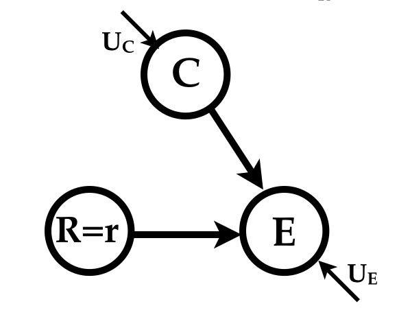
Commonsense tells Sol that clouds cause rain and that clouds cause a drop in energy production, while rain increases production by washing away the dirt on the panels. A graphical depiction (called the causal graph) of Sol’s mental model of the causal story hidden in the data is
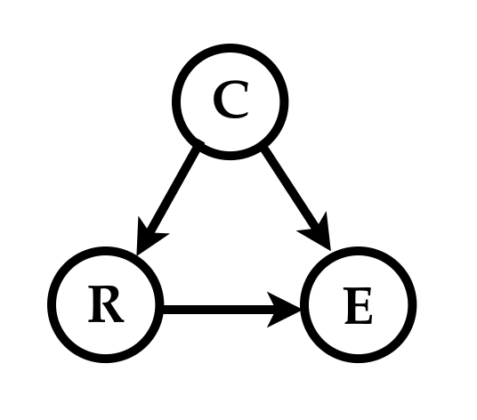
He estimates the necessary parameters of his causal model from the data, and implements his model as shown below to simulate behaviors or instances of the physical process (i.e, generate joint samples of \((C, R, E)\).
model = function(){
  c = runif(1, min=0, max=0.3)                         ## cloud-cover: C ~ Uniform(0, 0.3)
  r = floor(7 *(4*c^2 + runif(1, min=0, max=0.1)))     ## rainy-days: R = f_R(C, noise)
  e = 500 * (1 - 2*c + 0.1 * r) + 10 * rnorm(1)        ## energy: E = f_E(c, r, noise)
  return(data.frame(C=c, R=r, E=e))
}
Because the causal graph is a depiction of the sequential computation of the variables it must be a Directed Acyclic Graph (DAG) which defines a partial order on the variables.
Ignoring the particular functional forms we can notice that the order of computations follows the topological order of the variables in the graph above. The average cloudiness (\(C\)) is a random variable, the rainy days variable (\(R\)) is some function of \(C\) and noise, and the energy (\(E\)) is a function of \(C\), \(E\) and different noise. The noisy functions attempt to capture both measurement and modeling errors.
Note that because of the noise variables, the above program defines a joint distribution over the triple \((C, R, E)\). In fact, Sol can compute the conditional density \(P(E | R=r)\) by simply sampling from the simulator, filtering for \(R=r\) and fitting a density estimator to the energy values on the filtered samples. The conditional densities look as below
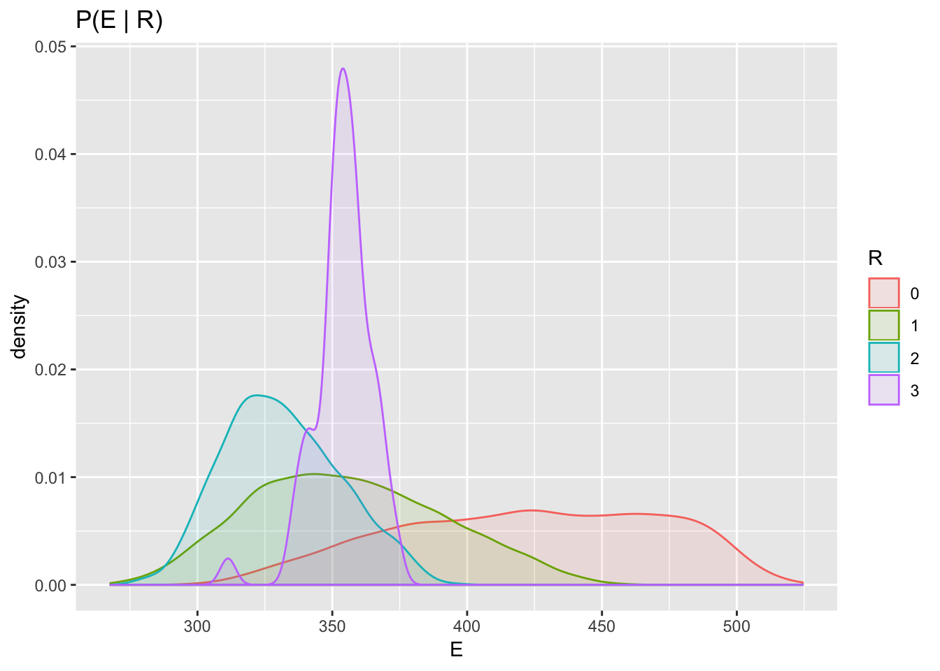
According to the distribution defined by the simulator the highest energy production tends to happen in weeks with no rain. This is perhaps mildly surpising for someone who hasn’t heard of confounding; the data shows this because both rain and energy are affected by their common cause – cloudiness. This implies that we cannot infer causation from the observed correlation between rain and energy production.
Sol rewrites his simulator making the noise variables explicit, as well as adding some optional arguments to override some of the computations as follows
model = function(do_c, do_r, do_e, do_uc, do_ur, do_ue){
  uc = ifelse(missing(do_uc), runif(1), do_uc)       ## Uc ~ Uniform(0, 1)
  c = ifelse(missing(do_c), uc * 0.3, do_c)          ## C = Uc * 0.3

  ur = ifelse(missing(do_ur), runif(1), do_ur)       ## Ur ~ Uniform(0, 1)
  r = ifelse(missing(do_r),
             floor(7 *(4*c^2 + ur * 0.1)), do_r)     ## R = f_R(C, Ur)

  ue = ifelse(missing(do_ue), rnorm(1), do_ue)       ## Ue ~ Normal(0, 1)
  e = ifelse(missing(do_e),
        500 * (1 - 2*c + 0.1 * r) + 10 * ue,
        do_e)                                        ## E = f_E(C, R, Ue)

  return(data.frame(C=c, R=r, E=e, UC=uc, UR=ur, UE=ue))
}

generate = function(num_samples, ...){
  df <- do.call(rbind, lapply(1:num_samples, function(i) model(...)))
  df$R <- factor(df$R, levels=0:3)
  df
}
Although the code now looks more complicated it implements exactly the same model as the version before it, albeit allowing Sol to arbitrarily set any of the variables to values of his choosing. Setting the function argument “do_x” allows Sol to surgically replace the value of variable \(X\) in his simulation from what it would have been otherwise. (The “generate” function is just a helper to sample from the simulator.)
The underlying model can more clearly be depicted as
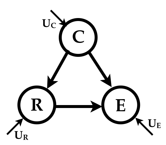
The randomness in the simulator is owed only to the indepdendent noise variables \(U_C\), \(U_R\) and \(U_E\); the variables \(C\), \(R\) and \(E\) are deterministic functions of the variables they listen to (to borrow a phrase that Judea Pearl populalized). We can think of the values taken by the noise variables \(U_C\), \(U_R\) and \(U_E\) for any sample as defining that sample. They give the sample its individuality as it were.
A model with this structure is termed a Structural Causal Model, which I only mention to prime you to its encounter in future wanderings. It is a probabilistic model with additional causal assumptions.
The awesome power conferred by a simulator in one’s possession brings a temptation to meddle that is hard to resist even for an old testament god, let alone a mere solar scientist. Sol dutifully proceeds to meddle.
Interventions
To determine the causal effect of rain on energy production, Sol needs to simulate the process in a parallel universe where rain can be controlled independently of its influence from cloudiness. (He is after all investigating the effect panel washing would have on energy production, and cloudiness would not affect the decision to wash.) He intervenes to set the rain variable to different values as follows
n <- 10000
## generate n samples each by setting do_r to different values 0, 1, 2, or 3
df_intervention <- do.call(rbind, lapply(0:3,function(r) generate(n, do_r = r)))
ggplot(aes(E, fill = R, color = R), data=df_intervention) + geom_density(alpha = 0.1)+ggtitle("P(E | do(R))")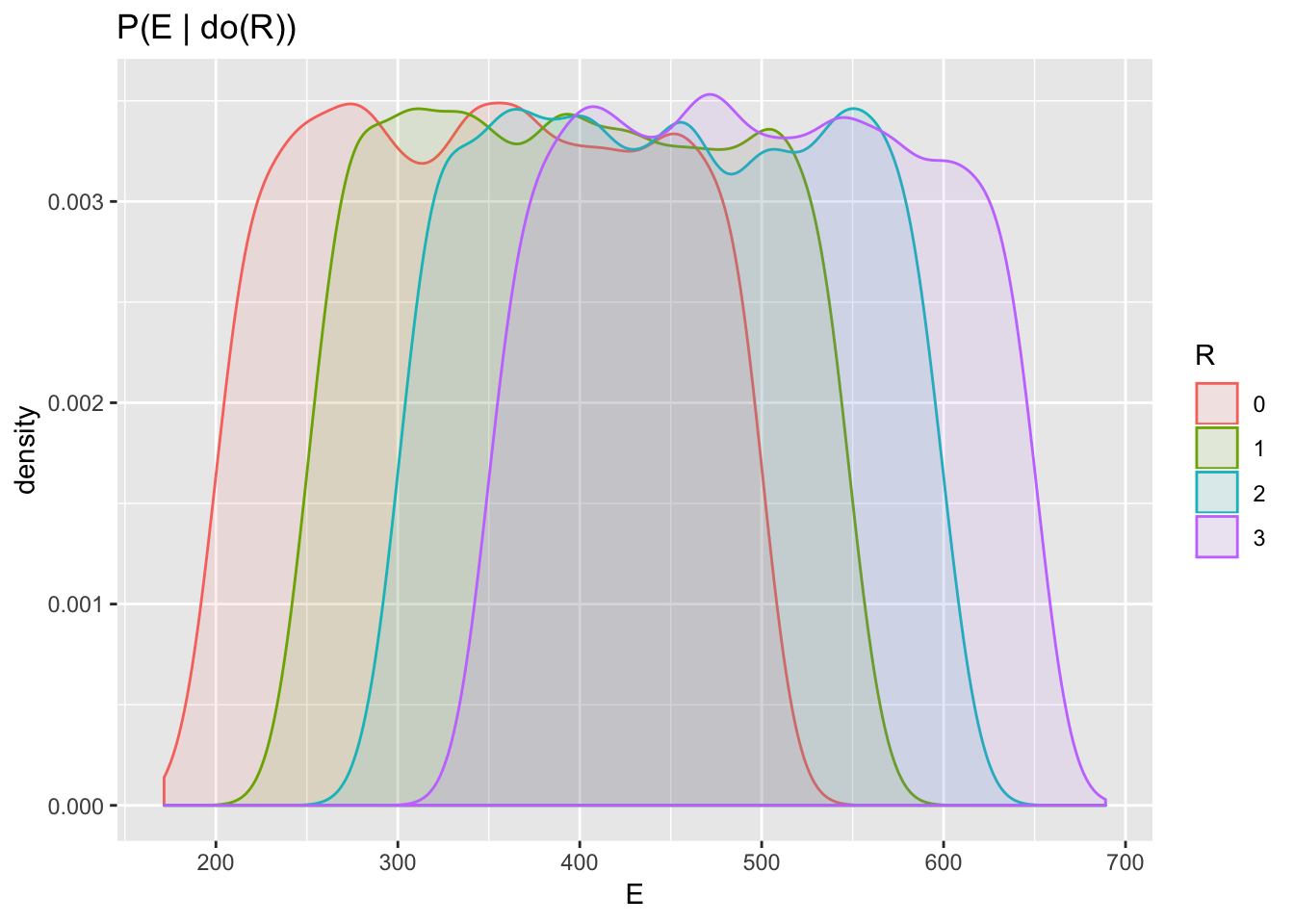
The quantity \(P(E|do(R=r))\) is shorthand for the distribution of \(E\) produced when Sol samples from his simulator by setting the “do_r” argument to the value \(r\).
Contrary to the conditional probabilities estimated before, this simulation shows that more rain causes more energy. The so-called interventional distribution \(P(E | do(R =r))\) is obtained by causal conditioning and is in general different from the Bayesian conditional distribution \(P(E|R=r)\).
A graphical representation of the way the process unfolds in the parallel universe (and of the program that simulates it) is
All the arrows pointing to the node \(R\) have been severed and its value is set to \(r\). This is the essence of what it means to intervene – we remove any other causal influences on the variable on which we are intervening. This is why Bayesian conditioning differs from causal conditioning – when we causally condition, we are hypothesizing a different universe which is running a different program, consequently producing a different distribution over the observables.
One way to internalize the conceptual difference between the two kinds of conditioning is to note that causal conditioning is carried out by setting the “do” argument of the simulator, whereas Bayesian conditioning is carried out by sampling and filtering. For example, to estimate \(P(E | do(R =r), C=c)\) we sample from the simulator by setting argument do_r to \(r\), then filter the generated samples for \(C =c\) and compute the histogram over \(E\) from the filtered samples.
So, what is the distribution of \(E\) given \(do(R=r)\)? First note that the joint probability \(P(E, C|do(R=r))\) can be computed as
\[\begin{align} P(E, C=c|do(R=r)) &= P(E|C=c, do(R=r)) P(C=c) \\ &= P(E|C=c, R=r) P(C=c) \\ \end{align}\]
The first equality stems from how \(E\) is generated by the simulator – first generate \(C\) according its marginal probability and then generate \(E\) from \(C\) and the “intervened” value of \(R\). The second equality results from the fact that if \(C\) were fixed, it does not matter whether \(R=r\) results “naturally” or from being intervened on.
Therefore \[P(E|do(R =r)) = \sum_c P(E, C=c|do(R=r)) = \sum_c P(E|C=c, R=r) P(C=c)\] This result is an instance of something called the backdoor formula about which I will have more to say in my next post. For now just notice how an expression for causal conditioning (with a “do”) was translated into an expression containing only Bayesian conditioning (without any “do”s).
Now might be a good juncture to break for rest and to take in the scenery. As a warmup for what is coming next you might want to mull the following questions. Looking at the order of the calculations in Sol’s simulator above may help.
- What is \(P(E | do(R=r), do(U_R=u_r))\)?
- How does \(P(E|do(C = c))\) relate \(P(E|C=c)\)?
- What is the interpretation of \(P(E|do(U_R = u_r))\)?
Counterfactuals
As noted above, for any one sample from the model, the particular values assumed by the random variables \(U_C\), \(U_R\) and \(U_E\) for that sample completely specify it, and together represent a particular week in our universe. In other words, we can define an individual week by assigning specific values to these random variables.
Let us generate a single sample from, Sol’s simulator.
set.seed(0)
week_a = generate(1)                     ## generate one sample
kable(week_a, format="html", digits = 2) ## print the sample| C | R | E | UC | UR | UE |
|---|---|---|---|---|---|
| 0.27 | 2 | 327.73 | 0.9 | 0.27 | -0.33 |
We can now ask the following question. What would the energy production have been in this week had it not rained at all? This is what we call a counterfactual; a question about events in a universe where they unfolded contrary to those in our actual factual universe.
What does this counterfactual question mean? Colloquially it means, “all else being equal how would the energy production \(E\) have changed to if we had set \(R\) to zero?”. Clearly the “all else” does not include \(E\) itself. We only mean that while not changing anything that gives this week its individuality how does intervening on \(R\) affect \(E\).
As we said before, an instance derives its individuality from the values assumed by the noise variables \(U_C\), \(U_R\) and \(U_E\). Therefore the way to answer the counterfactual is to run the simulator with the arguments do_uc, do_ur, do_ue set to 0.9, 0.27, and -0.33 respectively and to set do_r to 0.
counterfactual_week_a = generate(1, do_uc=0.9, do_ur=0.27, do_ue=-0.33, do_r=0)    ## counterfactual!
kable(counterfactual_week_a, format="html", digits = 2) | C | R | E | UC | UR | UE |
|---|---|---|---|---|---|
| 0.27 | 0 | 226.7 | 0.9 | 0.27 | -0.33 |
We estimate that the energy production would have been 227 Mwh ((instead of the 328 Mwh that was actually observed) had it not rained in that particular week. Note that because all the noise variables are fixed, there is no stochasticity left in the simulator – it would produce exactly the same vector of observations no matter how many times we run it.
We can perform this \(do(R=0)\) counterfactual computation for every instance in our universe. Because of the lack of stochasticity in counterfactual sample, there is a one-to-one correspondence between every example in the factual universe and those in the counterfactual universe.
I will annotate the column names of the counterfactual samples by a subscript “r” (or "_r" in the column names) to indicate that these measurements are made in the parallel universe where \(R\) was intervened on.
n = 10000
weeks_actual = generate(n)
weeks_counterfactual = do.call(rbind, lapply(1:n,function(i)
           generate(1, do_uc=weeks_actual$UC[i], do_ur=weeks_actual$UR[i], do_ue=weeks_actual$UE[i], do_r=0)))
names(weeks_counterfactual) = paste0(names(weeks_counterfactual), "_r") ## rename counterfactual variables
df_counterfactual = cbind(weeks_actual,weeks_counterfactual)
kable(df_counterfactual[1:10,], format="html", digits = 2) | C | R | E | UC | UR | UE | C_r | R_r | E_r | UC_r | UR_r | UE_r |
|---|---|---|---|---|---|---|---|---|---|---|---|
| 0.27 | 2 | 340.26 | 0.91 | 0.20 | 1.27 | 0.27 | 0 | 240.26 | 0.91 | 0.20 | 1.27 |
| 0.20 | 1 | 336.36 | 0.66 | 0.63 | -1.54 | 0.20 | 0 | 286.36 | 0.66 | 0.63 | -1.54 |
| 0.05 | 0 | 444.09 | 0.18 | 0.69 | -0.29 | 0.05 | 0 | 444.09 | 0.18 | 0.69 | -0.29 |
| 0.15 | 1 | 424.74 | 0.50 | 0.72 | 2.40 | 0.15 | 0 | 374.74 | 0.50 | 0.72 | 2.40 |
| 0.23 | 2 | 358.78 | 0.78 | 0.93 | -0.80 | 0.23 | 0 | 258.78 | 0.78 | 0.93 | -0.80 |
| 0.04 | 0 | 459.44 | 0.13 | 0.27 | -0.29 | 0.04 | 0 | 459.44 | 0.13 | 0.27 | -0.29 |
| 0.11 | 0 | 381.17 | 0.38 | 0.87 | -0.41 | 0.11 | 0 | 381.17 | 0.38 | 0.87 | -0.41 |
| 0.18 | 1 | 361.21 | 0.60 | 0.49 | -0.89 | 0.18 | 0 | 311.21 | 0.60 | 0.49 | -0.89 |
| 0.20 | 1 | 337.08 | 0.67 | 0.79 | -1.24 | 0.20 | 0 | 287.08 | 0.67 | 0.79 | -1.24 |
| 0.12 | 1 | 430.39 | 0.41 | 0.82 | 0.38 | 0.12 | 0 | 380.39 | 0.41 | 0.82 | 0.38 |
As we expect, for all cases where \(R=0\), the counterfactual values for all the variables equal their actual values (a no-rain week in our universe would see no difference in the counterfactual universe where we force it to not rain). Also since the noise variables in the counterfactual universe have the same values as those in ours the subscript "_r" is unnecessary.
Let us compare the causal conditional distribution \(P(E | do(R=0))\) with the distribution of the counterfactual energy variable \(E_r\) in the above table.
plot(density(df_intervention$E[df_intervention$R == 0]), col="blue",
     main = "R = 0", xlab = "E")
lines(density(df_counterfactual[["E_r"]]), col="red")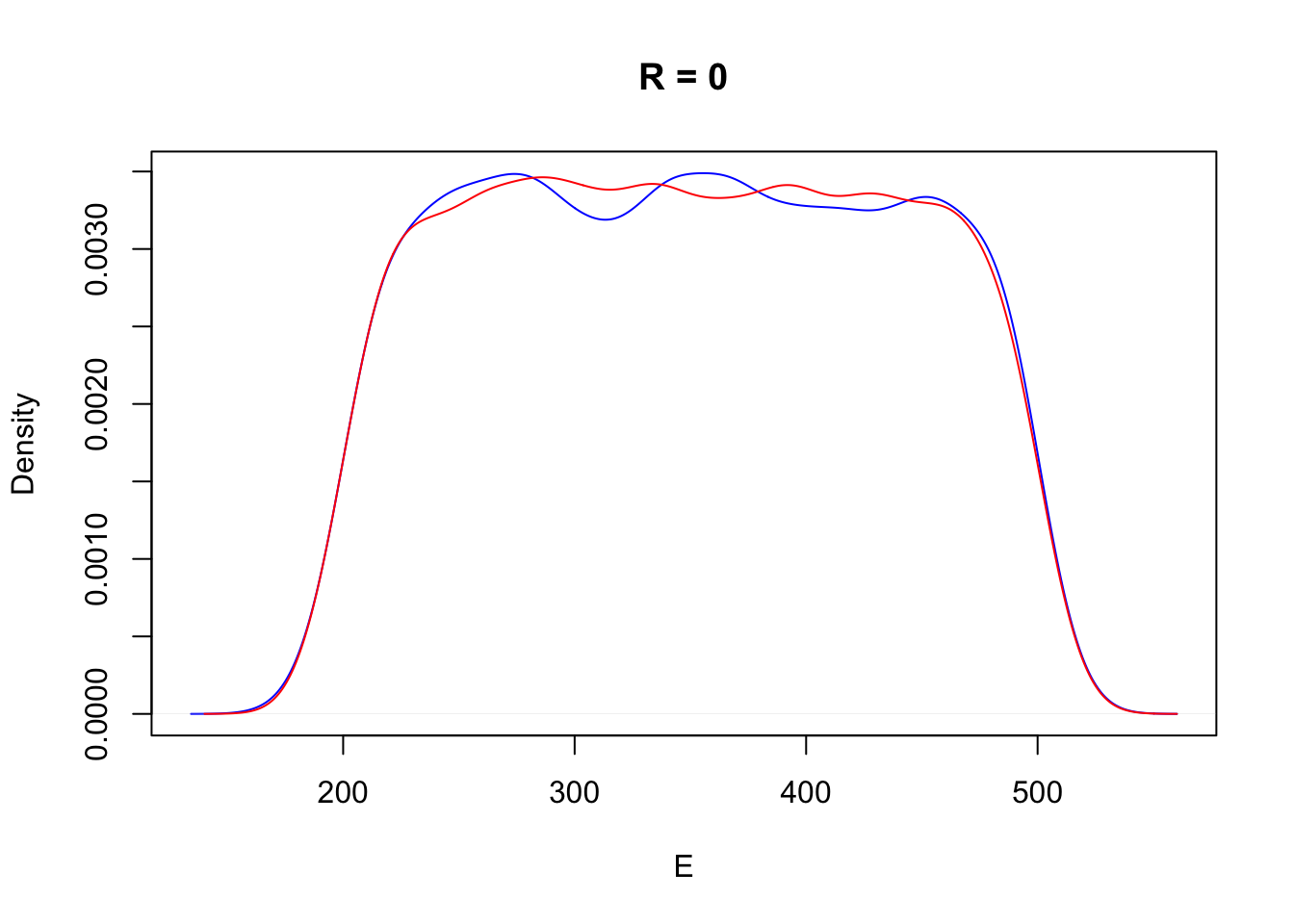
Perhaps surprisingly they turn out to be the same. A moment’s reflection about how these two distributions were generated from Sol’s simulator should convince you that the inteventional distribution obtained by causal conditioning is precisely the summary of counterfactuals over all the instances. In fact the interventional distribution \(P(E|do(R=r))\) could more precisely be written as \(P(E_r|R_r = r)\). (Note that this is non-standard notation but it makes it easier for me to keep everything straight.)
The notion of counterfactuals is therefore more fundamental than the notion of causal conditioning or interventional distributions. All interventional questions could be answered by generating counterfactual samples, and then appropriately conditioning and aggregating them.
We can ask very general conditional questions about this counterfactual universe. For example, “for a week with low energy production, what is the distribution of the decrease in energy production if we intervened to make it not rain?” Answer: \(P(E - E_r|R_r=0, E < e)\). Filter the above table for \(E < e\) and compute the histogram over the difference \(E-E_r\) on the remaining rows.
We have been asking counterfactual questions about instances generated from the simulator. What if Sol wanted take a particular week from his dataset and ask what the energy production would have been had it not rained in that week? Since he only has access to the \(C\), \(R\) and \(E\) variables for that week but not the noise (\(U_.\)) variables, he cannot follow our simple procedure of running simulator with arguments do_r=0 and do_uc, do_ur and do_ue set to the particular values. The procedure he needs to follow is to first estimate the posterior distribution over noise variables from the probabilistic model (which the simulator mirrors) conditioned on the observations for that week, and use samples from this posterior as arguments for the simulator. In pseudocode
sample_counterfactual(c, r, e){ ## single week observation = (c, r, e)
  for(i in 1:num_samples) {
    uc, ur, ue = sample_from(P(UC, UR, UE | C=c, R=r, E=e))
    counterfactual_samples_E[i] = generate(1, do_r=0, do_uc=uc, do_ur=ur, do_ue=ue)[["E"]]
  }
  return(counterfactual_samples_E)
}
Note that this procedure is no longer one-to-one; for a given week we obtain a distribution over the energy production in the counterfactual “no-rain” universe.
To summarize, the procedure to answer causal questions is to translate it into a description of the variables to fix in the simulator, and of how to filter and aggregate the generated samples.
In the happy situation where we have a fully-fledged causal probabilistic model (and hence a simulator) that can generate joint samples of all the variables in the physical process the preceeding discussion is (almost) the entire story.
Unhappy Situations
Regrettably we live in a universe where the demand for happiness outstrips supply. If a simulator of the physical process were not available to answer your counterfactuals, what else might be?
Graph known, data with all variables measured. This is a situation where you know all the variables that constitute the system, have observations for all of them, and also know the causal structure (the DAG). All you need to produce a simulator is to estimate the functions that compute a variable from its parents (and the variable specific noise) – the so-called mechanisms of the causal model. In a future post I will present an approach for end-to-end learning of all the causal mechanisms of a system.
Graph known, not all variables measured. This is where you will need do-calculus – a framework systematized chiefly by the work of Judea Pearl and his students. The calculus enables a completely algorithmisized analysis of the graph and your “do” question to tell you 1) whether your question can be answered from your incomplete data, 2) if it can, produce a formula in terms of your observed variables to answer the question, and 3) if it cannot, specify for which unmeasured variables you will need to collect data to make the question answerable. Please take a moment to recover your composure after this astonishing claim.
The R package “causaleffect” implements the do-calculus. (There is a similar python package called “dowhy”.) A simple demonstration of the power of the calculus follows.
library(igraph)
library(causaleffect)
g = graph.formula(C -+ R, R -+ E, C -+ E, simplify=F) ## the causal graph
causal.effect(y="E", x="R", G = g)      ## produce the formula for P(E | do(R))
## [1] "\\sum_{C}P(E|C,R)P(C)"Note that this is the same backdoor formula that we derived earlier by appealing to specific features of our simulator, which here was produced programmatically.
- Graph unknown, data with all variables measured. Estimating the causal structure is much easier if the data can be measured “actively”, that is, by actually intervening in the system that you are studying. This is not a luxury that is available in most circumstances. Several algorithms have been proposed that exploit the Markov independences implied by a causal structure (under another fairly mild assumption called faithfulness) to estimate (the estimable parts of) the causal graph from passively collected data.
- Graph unknown, not all variables measured. Even when not all the variables in the graph are measured, certain facts about the causal structure can be inferred from the incomplete data. I do not understand this topic well enough to say more.
- Graph unknown, no data. If you happen to find yourself in this situation, you should probably seek out a Bodhisattva to help with your counterfactual questions.
References
- If correlation doesn’t imply causation, then what does?, by Michael Nielsen. A excellent exposition of the basic concepts of causal calculus. A good place to start for the beginner.
- The Book of Why, by Judea Pearl & Dana Mackenzie. You would do well read this book by the father of modern causal reasoning intended for the popular audience.
- Lecture Notes, Cosma Shalizi. This is an excellent resource for slightly more technical material but presented in a very engaging manner, not only about causality but other statistical topics.