Do-calculus, Judea Pearl’s comprehensive algorithmic framework for causal reasoning, can intimidate even a seasoned statistician. I will try to present an intuitive justification of a couple of its common patterns – namely the back-door and, the seemingly magical, front-door adjustment formulas. Along the way I will derive the front-door formula (for a special case) from the back-door formula without invoking the rules of do-calculus.
In a previous post I attempted to explain the distinction between Bayesian and causal (or interventional) conditioning by introducing the do notation. In that solar panel washing story the scientist was able to construct a simulator for the data generating process, and answer interventional and counterfactual questions by appropriately manipulating the simulator. We cannot in general follow this procedure. In particular when not all variables are measured, even if we know the causal graph underlying the system under study, we will not be able to estimate all the mechanisms necessary to implement the simulator.
Confounding and Controlling
Let us tell a different story to illustrate the problem. Imagine an inventive statistician Ada working for a school district and trying to answer the following question: will introducing computer programming to the elementary school curriculum have a sufficiently beneficial effect on the students’ math proficiency in middle school to justify the additional cost?
Ada obtains a compilation of grade-level curriculum and aggregated proficiency data for school districts across the country. She notices in the data that most school districts offer some number of optional after-school programming classes to their elementary students. A quick analysis shows her that indeed the middle schools that are in neigborhoods where elementary schools offer more of these classes have higher standardized math scores.
However, Ada suspects that part of the effect is due to a common cause: perhaps districts where schools offer more programming classes have more progressive administrators and their imaginative curriculum design independently benefits middle school math proficiency. Let us call this so-called causal confounder “curriculum creativity” and denote it by the variable \(C\). Further let us denote the number of elementary school programming classes by \(P\), and middle school math proficiency by \(M\).
The causal diagram (the directed acyclic graph) that depicts Ada’s causal hypotheses is
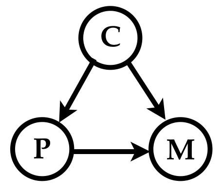
She knows that if the data she has in her possession has measurements of curriculum creativity \(C\), she should control for that variable to accurately estimate the causal influence of \(P\) on \(M\).
What does such controlling entail? In the language of modern causal reasoning she wishes to estimate the interventional probability \(Pr(M|do(P =p))\), i.e., the probability of math proficiency \(M\) if she were to intervene and set the number of programming classes to \(p\) independent of its causal influence from \(C\).
That is, to answer the causal query she needs to sever the causal link between \(C\) and \(P\) present in real-world process that generated her data, and hypothesize a data generating simulator that resembles the real-world process in all aspects but for that surgery.
To generate an example from the world where she had intervened to set \(P=p\), the hypothesized simulator first generates \(C = c\) according to its prior, and then generates \(M\) according to the probability \(P(M | C=c, P=p)\). Therefore the joint distribution \(Pr(M, C=c|do(P=p))\) is given by \[ Pr(M, C=c| do(P=p)) = Pr(M| C=c, P=p) Pr(C=c)\]
The interventional probability \(Pr(M|do(P =p))\) is obtained by marginalizing out \(C\) from this expression as \[Pr(M|do(P =p)) = \sum_c Pr(M| C=c, P=p) Pr(C=c)\] For Ada’s problem, this is the back-door formula, and is precisely what she needs to calculate to control for the confounder \(C\).
The path \(P \textrm{--} C \textrm{--} M\) is called a backdoor path from \(P\) to \(M\): an undirected path from \(P\) to \(M\), with an arrow pointing into \(P\). Such a backdoor path indicates possible confounding. To answer causal questions in a general causal graph, all backdoor paths need to be blocked by controlling for some set of variables \(S\) that satisfy the backdoor criterion, viz., every backdoor path must pass through some variable in \(S\), and \(S\) should not include any descendent of the variable on which we are intervening.
(The above paragraph paraphrases Cosma Shalizi’s lecture notes, which present more thorough exposition of the topic and a formal derivation of the back-door formula.)
Unobserved Confounder
The reason \(C\) confounds the causal effect of \(P\) on \(M\) (and for needing to control for it) is because even if we observed a very strong correlation between \(P\) and \(M\) we cannot distinguish between a large causal effect of higher availability of programming classes on math scores, and the effect being entirely due to the curriculum creativity.
Unfortunately for Ada her data lacks any measurements of the creativity of the curriculum at different school districts (even if such a thing could be measured), leaving her in the hazy world of unmeasured confounding where she cannot apply the back-door formula to estimate the interventional probability. However, she notices that her data contains measurements of the student enrollment rates in the optional programming classes. She hypothesizes that the causal diagram including the enrollment variable \(E\) looks like so
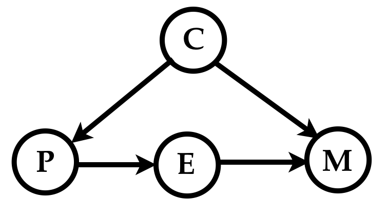
The above diagram encodes Ada’s causal story that math proficiency is affected by programming classes only through their corresponding enrollment rates, and that the enrollment rates themselves are not directly affected by curriculum creativity. Stated differently Ada assumes that the enrollment rate \(E\) blocks the only causal path between \(P\) and \(M\), and the only path from curriculum creativity \(C\) to enrollment rates \(E\) is blocked by the number of programming classes \(P\).
From her causal story Ada reasons as follows.
"Even though the data shows strong correlation between \(P\) and \(M\), not knowing \(C\) prevents me from distinguishing between the two extremes: 1) \(M\) is independent of \(C\) given \(P\), i.e., there is no direct effect of curriculum creativity on math scores, and 2) \(M\) is independent of \(P\) given \(C\), i.e., the entirety of the statistical dependence of \(M\) on \(P\) is due to the common parent \(C\) implying no causal effect of programming classes on math scores.
"However, even though districts with more programming classes have better math performance, I should notice in the data that districts with the similar number of programming classes but with different enrollment rates have similar math scores, it would tell me that the programming classes did not cause the better math scores.
"Similarly if districts that offer no programming classes have similar math scores as the districts that offer a lot of classes but have zero enrollment, I would know that of curriculum creativity did not cause the high math scores in districts with many programming classes and high enrollment.
“In other words, at least in these edge cases, the measurement of \(E\) would help me distinguish between the above two causal extremes, even though \(C\) was not measured!”
Ada’s reasoning applies more broadly. Specifically, under the model defined by her causal graph, the interventional probablity \(Pr(M|do(P))\) can be written in terms of only the joint distribution over the variables \(P, E\) and \(M\) yielding the front-door formula. The particular structure of her causal model allows Ada to use the measurements of \(E\) to deconfound the causal question without needing to measure \(C\).
Front-Door Formula
If we accept the veracity of the back-door formula above, we can derive the front-door formula from it using only the rules of probability, which I find more intuitive than arriving at it using the do-calculus. The following 8 lines show the derivation, with parts where the action took place shown in blue. Remember that we are searching for a formula for \(P(M|do(P=p))\) where the variable \(C\) does not appear.
\[\begin{eqnarray} Pr(M | do(P = p)) &=& \sum_c Pr(M | P=p, C=c) Pr(C = c) \\ &=& \sum_c \color{blue}{\sum_e Pr(M, E=e | P=p, C=c)} Pr(C = c) \\ &=& \sum_c \sum_e \color{blue}{Pr(M| E=e, C=c) Pr(E=e|P=p, C=c)} Pr(C = c) \\ &=& \sum_c \sum_e Pr(M| E=e, C=c) \color{blue}{Pr(E=e|P=p)} Pr(C = c) \\ &=& \sum_c \sum_e Pr(M| E=e, C=c) Pr(E=e|P=p) \color{blue}{\sum_{p'} Pr(C = c|P=p') Pr(P=p')} \\ &=& \sum_c \sum_e \color{blue}{\sum_{p'}} Pr(M| \color{blue}{P=p'}, E=e, C=c) Pr(C=c | P=p', \color{blue}{E=e}) Pr(E=e|P=p) Pr(P=p') \\ &=& \sum_e \sum_{p'} \color{blue}{\sum_{c} Pr(M, C=c| P=p', E=e)} Pr(E=e|P=p) Pr(P=p') \\ &=& \sum_e \sum_{p'} \color{blue} {Pr(M| P=p', E=e)} Pr(E=e|P=p) Pr(P=p') \end{eqnarray}\]
Let us look at the derivation a line at a time. Before we do that let us notice two facts about the probability distribution defined by Ada’s causal graph – 1) knowing only \(P\) renders \(C\) and \(E\) independent, and 2) knowing \(C\) and \(E\) makes \(M\) independent of \(P\).
- The first line is just the back-door formula from earlier.
- The second line writes the probability \(Pr(M|P, C)\) as the marginalization over the joint probability \(Pr(M, E|P, C)\).
- The third line writes the joint \(Pr(M, E|P, C)\) as the product of the conditional probability \(Pr(M|E, P, C)\) and \(Pr(E|P, C)\).
- The fourth line uses the fact that \(E\) and \(C\) are independent given \(P\). This is the first step that uses the properties of Ada’s graph.
- The fifth line creates an auxiliary index \(p'\) over the values of \(P\) and writes the probability \(Pr(C)\) as the marginalization over \(Pr(C, P)\). I know to do this because I know where we are headed having seen the front-door formula before.
- Line 6 does a few things. First we use the fact that that \(M\) is independent of \(P\) when \(C\) and \(E\) are known to rewrite \(P(M|E, C)\) as \(P(M|P, E, C)\). Second, we again use the conditional independence of \(C\) and \(E\) to rewrite \(Pr(C|P)\) as \(Pr(C|P, E)\). Finally we move the summation over \(p'\) outside.
- Line 7 simply collects the product of \(Pr(M|P, E, C)\) and \(Pr(C|P, E)\) as the joint \(Pr(M, C|P, E)\) and reorder the summations.
- Line 8 marginalizes out \(C\) from the joint \(Pr(M, C|P, E)\) yielding the front-door formula without any term containing \(C\), which is what we seek.
References
1.After trying to do it on your own, if you want to learn how to derive the front-door formula using do-calculus see Michael Nielsen’s blog post If correlation doesn’t imply causation, then what does?.